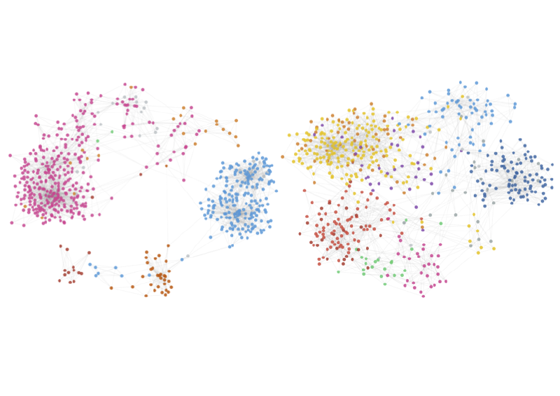
This project uses Graph Theory to analyze voting patterns in the French National Assembly. By treating MPs as nodes and voting similarity as edges, we map how MPs vote relative to each other, within and across political groups.
1. Introduction and political context
1.1 Institutional framework
The French National Assembly is the lower chamber of the French bicameral parliament. It is composed of 577 Members of Parliament elected for five years by a two-round single-member majority system, in 577 constituencies (566 in France, 11 for French citizens living abroad). Each Member of Parliament (MP) in the National Assembly is affiliated with a specific political group.
For illustrative purposes, Figure 1 presents the composition of three consecutive legislatures by political group:
| 14th Legislature | 15th Legislature | 16th Legislature |
|---|---|---|
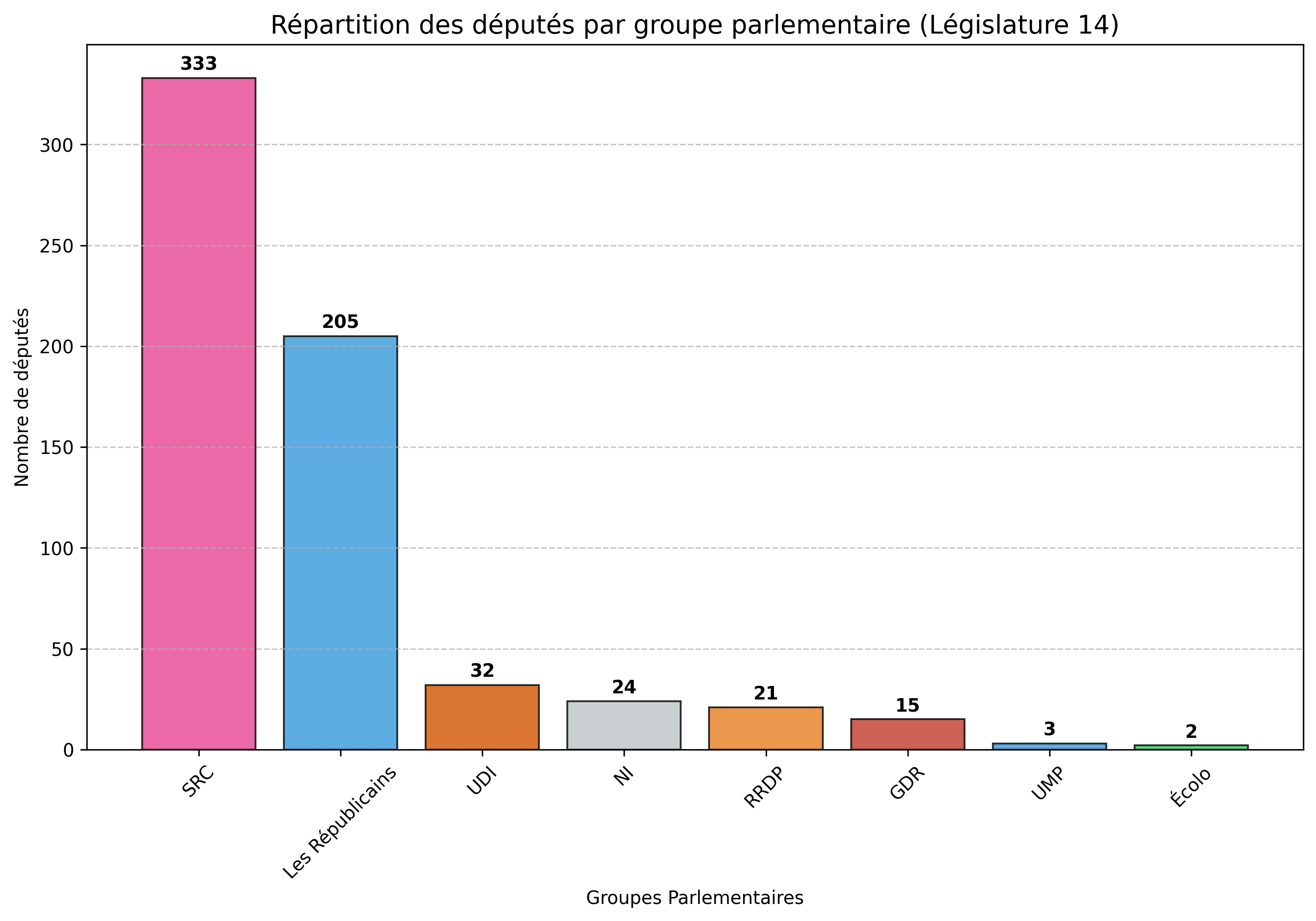 | 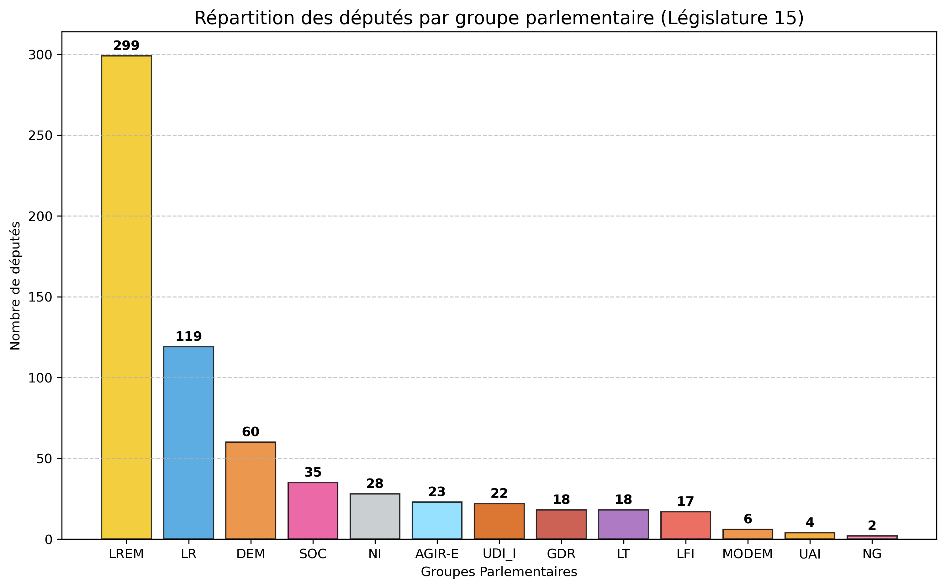 | 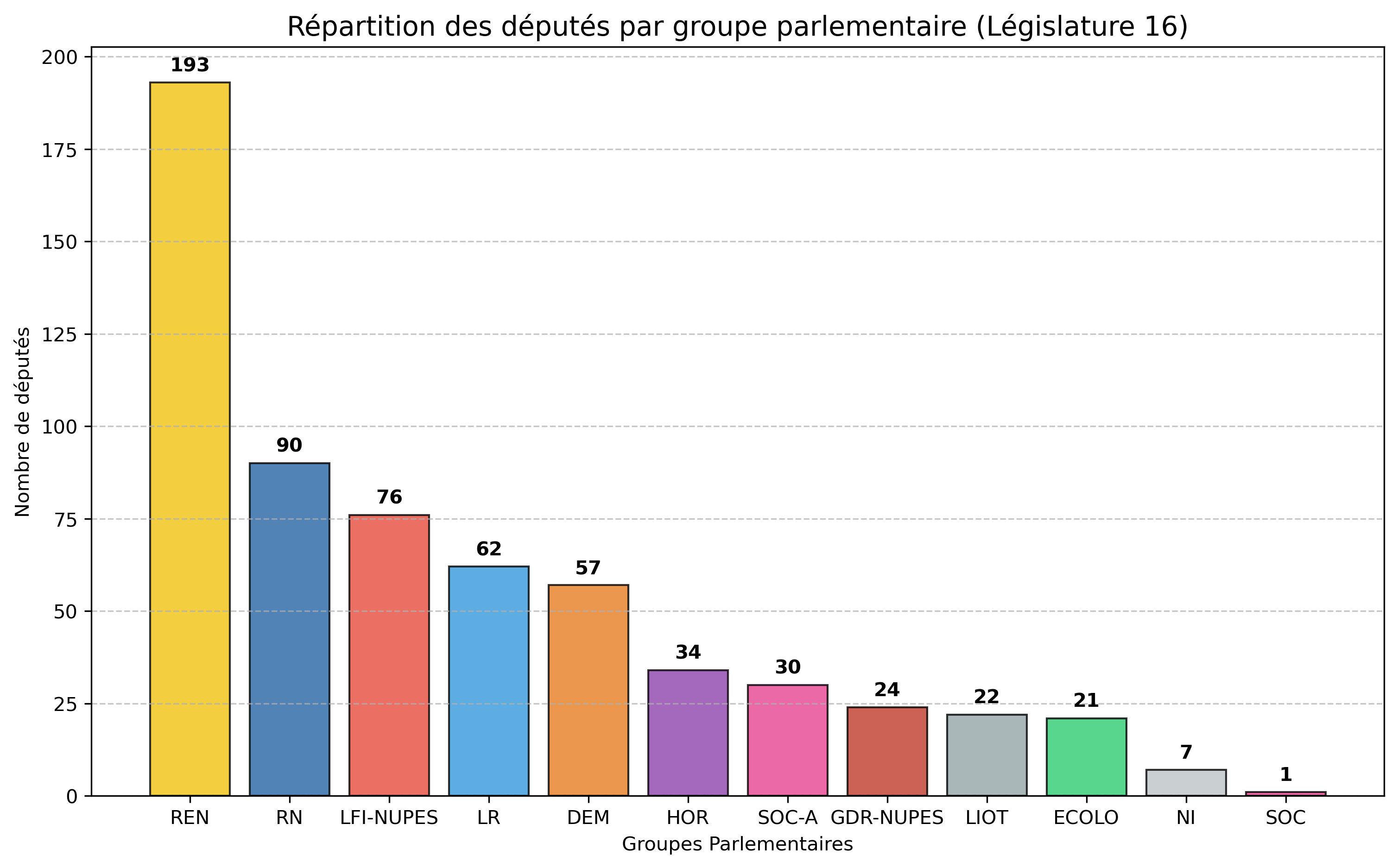 |
Figure 1: Distribution of the 577 Members of Parliament by political group.
We have more than 577 MPs because of resignations and replacements during the legislature.
1.2 Motivations and research questions
The objective of this project is to map the various political currents and their relative positioning by leveraging parliamentary voting data. Several questions naturally arise:
- What is the true ideological landscape beyond group labels?
- Does the historical left-right divide still exist?
- How has this structure changed between two major legislatures?
Our approach:
- Treats each ballot vote as a dimension in a political vector space
- Uses cosine similarity as a similarity metric
- Applies spatialization techniques (force-directed layout) and principal component analysis to visualize these data.
1.3 Overview of main political forces
To facilitate the interpretation of the spatialization graphs, the table below summarizes the main political groups, their associated colors in our study, and their core principles according to their official platforms.
| Color | Party/Group | Brief Description (Official Stance) | Source |
|---|---|---|---|
 | LFI / LFI-NUPES | Focuses on ecological planning, wealth redistribution, and a constitutional shift to a 6th Republic. | lafranceinsoumise.fr |
 | ECOLO | Advocates for environmental sustainability, social-ecology, and biodiversity protection. | lesecologistes.fr |
 | SRC / SER / SOC | Social-democratic model, defense of public services, and labor rights (Historical Socialist groups). | parti-socialiste.fr |
 | GDR | Defense of the working class, social justice, and opposition to liberal economic policies. | pcf.fr |
 | REN / LREM | Supports economic competitiveness, full employment policies, and European integration. | parti-renaissance.fr |
 | DEM / RRDP | Centrist approach, institutional balance, and education (includes center-left Radicals). | mouvementdemocrate.fr |
 | HOR | Focuses on long-term national stability, security, and supporting the presidential majority. | horizonsleparti.fr |
 | UMP / LR | Advocates for fiscal discipline, restoration of state authority, and economic liberalism. | republicains.fr |
 | RN | Prioritizes national sovereignty, immigration control, and national priority policies. | rassemblementnational.fr |
 | UDI / UAI | Liberal-humanist and pro-European project centered on a social-market economy. | parti-udi.fr |
 | LIOT | An independent group focused on territorial interests, decentralization, and local governance. | groupe-liot.fr |
 | NI | Non-affiliated members who do not belong to any parliamentary group. | assemblee-nationale.fr |
Note: Descriptions are synthesized from the “Manifesto” or “Our Values” sections of the parties’ official websites to ensure alignment with their self-defined political identity.
2. Framework and methodology
2.1 Vector representation of votes
2.1.1 The space of parliamentary votes
Each Member of Parliament can be represented by a vote vector $\mathbf{v}_i \in \mathbb{R}^n$, where $n$ is the number of ballot votes analyzed. Formally:
$$ \mathbf{v}_i = (v_{i,1}, v_{i,2}, \ldots, v_{i,n}) $$Each component $v_{i,j}$ encodes the MP’s position on a specific vote $j$:
- $+1$ : In favor (Vote for the motion)
- $-1$ : Against (Vote against the motion)
- $0$ : Abstention (Present but did not take a position)
- $\text{NaN}$ : No recorded vote (absent, or present without voting)
2.1.2 Vote matrix and data structure
After collecting votes via the NosDéputés.fr API, we construct a vote matrix $M \in \mathbb{R}^{m \times n}$:
- $m$ = number of MPs
- $n$ = number of ballot votes.
Each row corresponds to an MP’s vote vector, and each column corresponds to a specific vote.
$$ M = \begin{pmatrix} v_{1,1} & v_{1,2} & \cdots & v_{1,n} \\ v_{2,1} & v_{2,2} & \cdots & v_{2,n} \\ \vdots & \vdots & \ddots & \vdots \\ v_{m,1} & v_{m,2} & \cdots & v_{m,n} \end{pmatrix} $$Note on data: Most decisions in the Assembly are taken by show of hands, and no individual position is recorded. Only a public ballot (scrutin public) records each MP’s vote - for, against, abstention - and it is held only when mandatory (motions of censure, final reading of organic laws) or requested by the president of the sitting, the government, the committee responsible, or a group chair. These are the ballots the NosDéputés.fr API returns: our $n$ columns are public ballots, not all the votes held in the chamber.
So $\text{NaN}$ means “no vote recorded in a public ballot”, not “absent” - in either direction: a present MP need not take part, and an absent one can be covered by a proxy. The lowest participation figures are usually institutional rather than a sign of absenteeism: the President of the Assembly by convention rarely votes (Yaël Braun-Pivet, 0.15% of the ballots of the 16th Legislature), and an MP appointed to the government cannot vote for a month, then loses the seat to their substitute - Carole Grandjean and Clément Beaune, ministers from July 2022 to January 2024, are the next two lowest.
2.2 Handling missing data
Major challenge: The matrix $M$ contains missing values (NaN), corresponding to ballots where the MP’s vote was not recorded.
Two analytical frameworks are considered:
- “Presence-Only” (Pearson, Agreement Ratio): Measures agreement on the ballots both MPs voted on. It does not depend on the total volume of activity, but rests on few ballots when participation is low.
- “Volume-Aware” (Cosine, Jaccard): Integrates the level of activity into the geometry. By treating absence as a null component ($0$), it stabilizes the positions of inactive MPs by preventing them from reaching extreme similarity scores based on a single shared vote.
2.3 Four similarity metrics
2.3.1 Cosine similarity (chosen approach)
Cosine similarity measures the directional alignment between two vectors:
$$ S_{\cos}(\mathbf{A}, \mathbf{B}) = \frac{\mathbf{A} \cdot \mathbf{B}}{\|\mathbf{A}\| \cdot \|\mathbf{B}\|} = \frac{\sum_{j=1}^{n} A_j B_j}{\sqrt{\sum_{j=1}^{n} A_j^2} \sqrt{\sum_{j=1}^{n} B_j^2}} $$Implementation: NaN values are imputed as $0$.
Justification:
- Numerator: each ballot where both MPs voted the same way (for/for or against/against) adds $+1$, each ballot where they voted in opposite ways adds $-1$, and a ballot where either abstained or has no recorded vote adds $0$.
- Denominator: divides by the length of each vote vector, so the result depends on the direction of the vectors rather than on their length.
Properties:
- Range: $S_{\cos} \in [-1, +1]$.
- The result still depends on which ballots each MP voted on: two MPs who never voted on the same ballots have a similarity of $0$.
2.3.2 Pearson correlation
$$ \rho(\mathbf{A}, \mathbf{B}) = \frac{\mathbb{E}[(\mathbf{A} - \bar{A})(\mathbf{B} - \bar{B})]}{\sigma_A \sigma_B} $$NaN handling: Pairwise deletion.
Limitation: with pairwise deletion, the correlation is computed on the ballots both MPs voted on. If two MPs coincide on only a few votes and agree, Pearson can yield a perfect correlation ($+1.0$) based on very few ballots.
2.3.3 Jaccard similarity
$$ S_{\text{Jaccard}} = \frac{|\text{Agreements}|}{|P_A \cup P_B|} $$where $P_A$ and $P_B$ are the sets of votes where MPs A and B were present.
Problem: The union in the denominator lowers the similarity of two MPs with different activity levels, even if they agree on 100% of the ballots they both voted on.
2.3.4 Weighted agreement
$$ S_{\text{agreement}} = \frac{|\text{Agreements}|}{|P_A \cap P_B|} $$Problem: many pairs of MPs from the same group agree on every ballot they both voted on ($S = 1.0$): in the 16th Legislature, 11% of Renaissance pairs, 16% of LFI pairs and 1% of RN pairs. The metric then separates members of the same group poorly.
2.4 Synthesis: choice of metric
For this study, we use cosine similarity. Unlike Pearson, it does not give high similarities based on very few shared ballots. Unlike the Agreement Ratio, differences in which ballots MPs voted on, and individual deviations, translate into different similarities.
3. Voting network
3.1 Graph construction via k-NN
Rather than creating a complete graph (potentially 150k+ edges), we use a k-nearest neighbors topology:
For each Member of Parliament $i$:
- Compute $S_{\cos}(i, j)$ for all other MPs $j$
- Retain the $k = 5$ neighbors with the highest similarity
- Add a weighted edge $(i, j)$ with weight = $S_{\cos}(i, j)$
3.2 Layout algorithm: spring model
To spatialize the graph in 2D, we apply the Fruchterman–Reingold algorithm (force-directed layout). All MPs are thrown randomly onto the plot, and the algorithm iteratively adjusts their positions, driven by two competing forces. At each iteration every MP moves in the direction of the resulting force, by a distance that decreases linearly, so the layout gradually freezes. The figures below use at most 400 iterations (the computation stops at iteration 392 or 393, when the moves become negligible) and a fixed random seed.
$$ F_{\text{rep}}(i, j) = \frac{k^2}{d_{ij}} $$$$ F_{\text{attr}}(i, j) = \text{weight}_{ij} \cdot \left(-\frac{d_{ij}^2}{k}\right) $$These are the forces of Fruchterman and Reingold (1991). As in networkx, the attraction is multiplied by the weight of the edge, and applies only to linked MPs.
where:
- $\text{weight}_{ij}$ = The Cosine Similarity between MP $i$ and MP $j$. The more they vote alike, the stronger the pull.
- $F_{\text{rep}}$ = repulsion (every node pushes others away to avoid clutter).
- $F_{\text{attr}}$ = attraction
- $d_{ij}$ = Euclidean distance between MP $i$ and MP $j$ on the 2D map.
- $k$: the optimal distance between nodes ($k = 0.15$ here). It changes the spacing of the map, and therefore the layout.
For Linked MPs (The Top 5 Neighbors): the attraction grows with the similarity weight, so two linked MPs with a high similarity tend to end up close to each other.
For Non-Linked MPs (Everyone else): the distance $d_{ij}$ does not directly reflect their similarity. The algorithm doesn’t see the similarity between two MPs who aren’t in each other’s Top 5. Their distance on the map results from the repulsion force ($F_{\text{rep}}$) and from the chains of links attaching each of them to their own cluster: two MPs whose clusters share no links end up far apart, without the algorithm having compared them directly.
Reading the map:
- Clusters: MPs whose nearest neighbours belong to their own group form dense, color-coded clouds.
- Between clusters: MPs whose nearest neighbours belong to several groups are positioned between these clouds.
| 14th Legislature (2012-2017) | 15th Legislature (2017-2022) | 16th Legislature (2022-2024) |
|---|---|---|
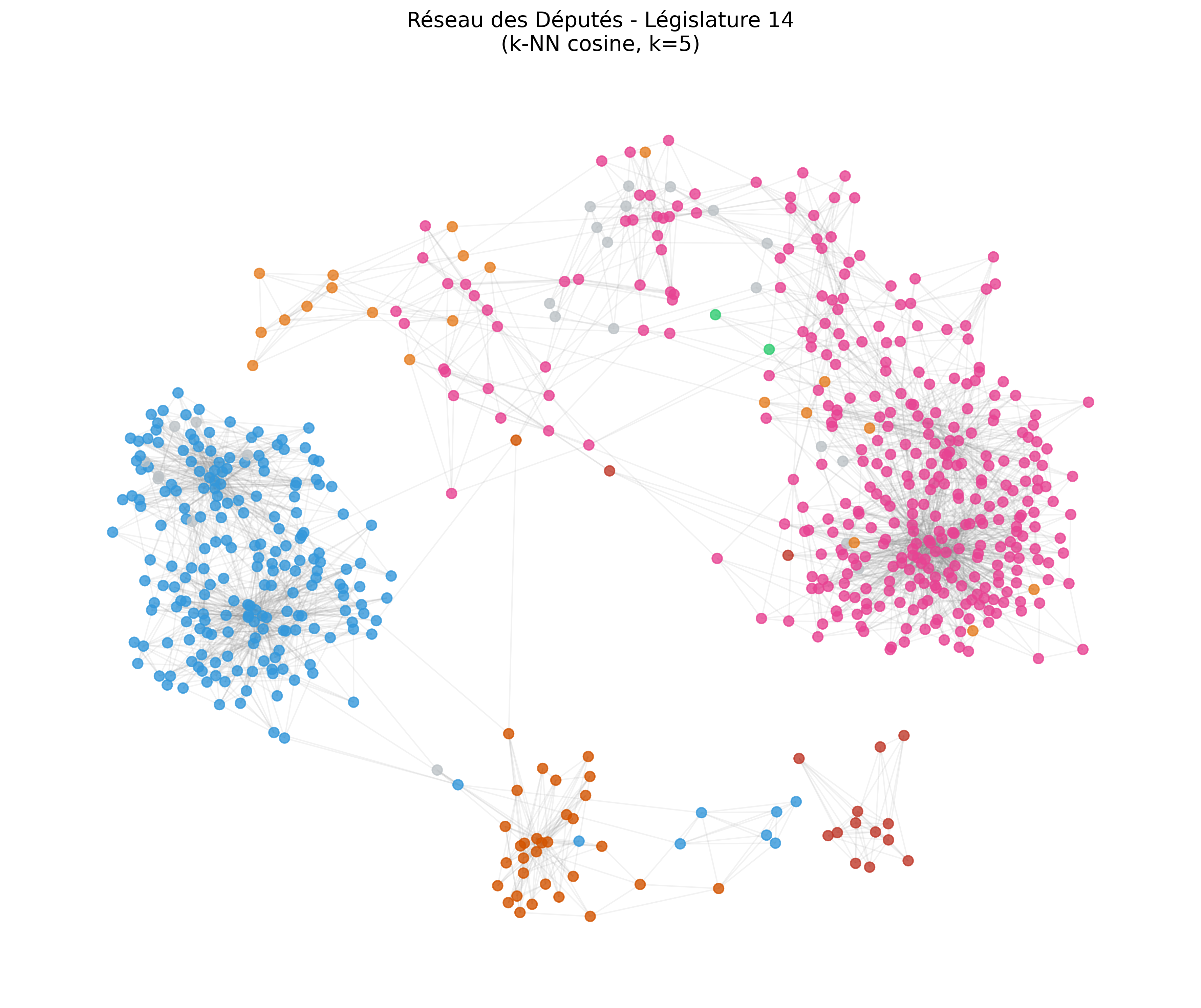 | 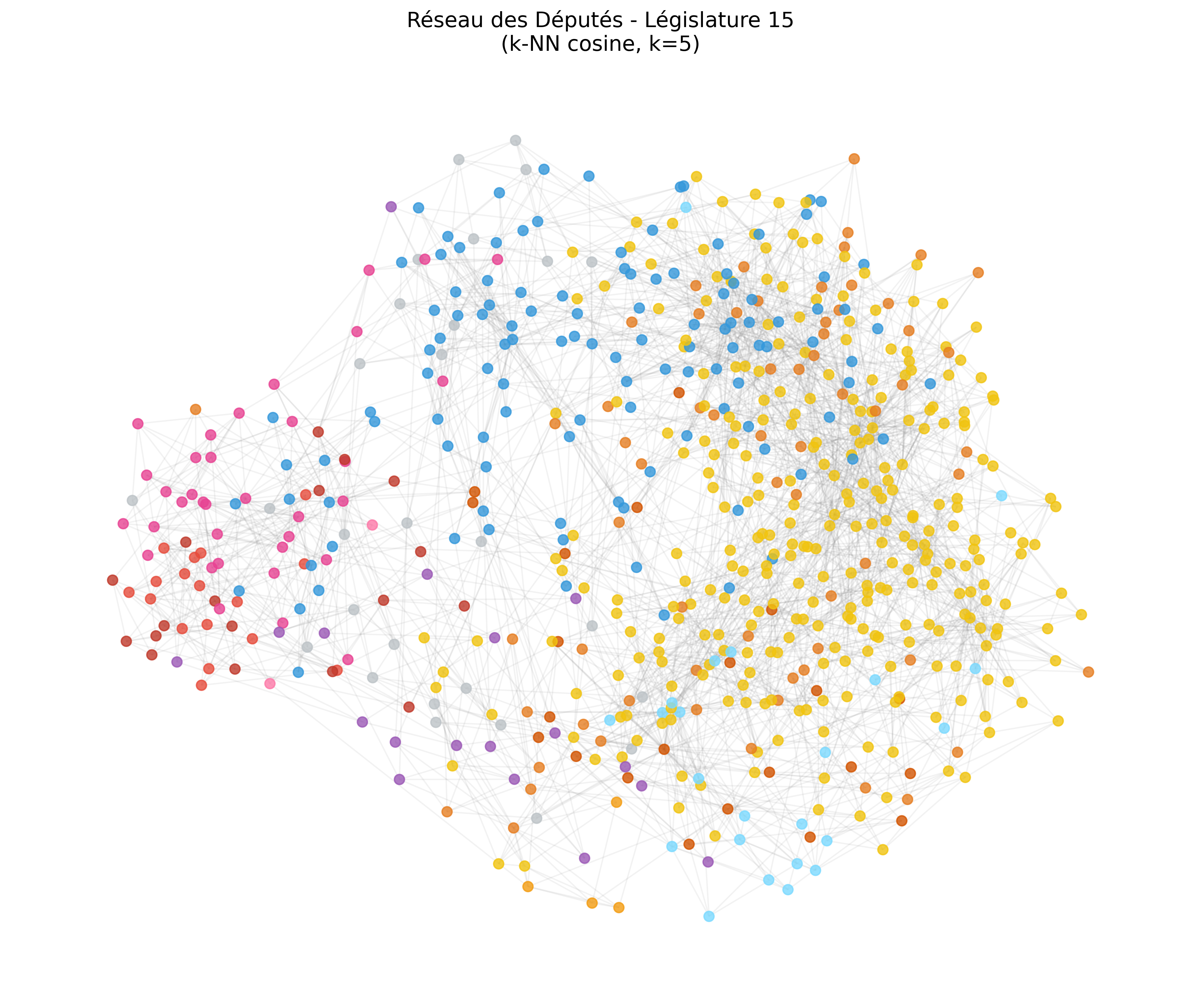 | 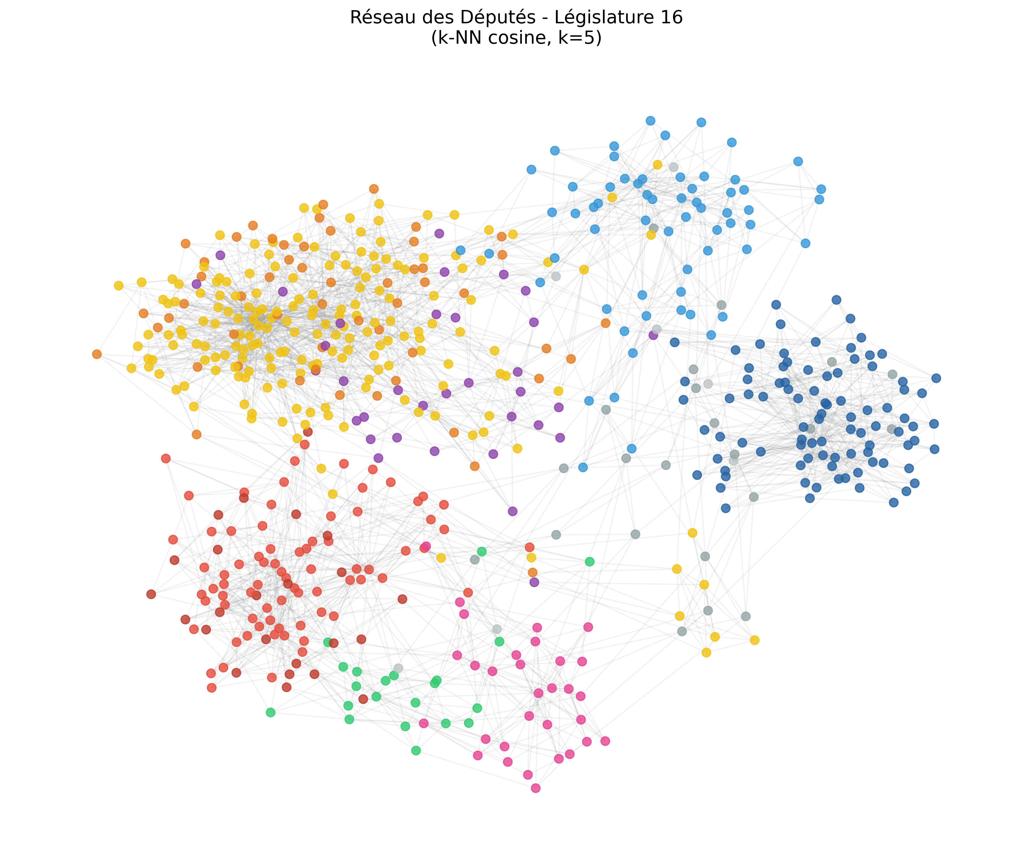 |
Figure 2: Graph of the 14th, 15th, and 16th legislatures using cosine similarity. Nodes are colored by political group. In the 14th Legislature, 13 of the 15 GDR MPs are linked only to each other: they form a component disconnected from the rest of the graph (top of the figure), whose position relative to the other MPs is arbitrary.
4. Principal component analysis (PCA)
We saw in section 2.1 that each MP is represented by a vote vector in a high-dimensional space ($\mathbb{R}^n$ where $n$ is the number of ballot votes). To visualize this $n$-dimensional voting space, we apply Principal Component Analysis (PCA). This dimensionality reduction technique projects the voting vectors onto a 2D plane (PC1 and PC2), preserving the maximum variance. Two deputies appearing close on the plot tend to have similar voting records, within the limits of a 2D projection (see 4.2).
4.1 Foundations of PCA
Formally, let $\mathbf{M} \in \mathbb{R}^{m \times n}$ be the voting matrix (with $m$ MPs and $n$ votes). We first transform it into a standardized matrix $\mathbf{X}_{\text{std}}$ where each element $x_{i,j}$ is defined as:
$$x_{i,j} = \frac{m_{i,j} - \mu_j}{\sigma_j}$$Where:
- $m_{i,j}$: The vote of MP $i$ for ballot $j$ (Abstention = 0).
- $\mu_j$: The mean vote for ballot $j$: $\mu_j = \frac{1}{m} \sum_{i=1}^{m} m_{i,j}$.
- $\sigma_j$: The standard deviation of ballot $j$: $\sigma_j = \sqrt{\frac{1}{m} \sum_{i=1}^{m} (m_{i,j} - \mu_j)^2}$.
1. Finding the principal axes
PCA identifies the two principal axes $\mathbf{u}_1, \mathbf{u}_2$ that maximize the explained variance. In other words, it looks for the directions along which the MPs are the most spread out:
$$ \mathbf{u}_k = \arg\max_{\|\mathbf{u}\|=1} \text{Var}(\mathbf{X}_{\text{std}} \mathbf{u}) $$2. Geometric projection
Each MP’s standardized vector $\mathbf{x_i} \in \mathbb{R}^n$ is projected onto this plane to obtain their 2D coordinates $(z_{i,1}, z_{i,2})$:
$$ z_{i,1} = \mathbf{x_i} \cdot \mathbf{u_1}, \quad z_{i,2} = \mathbf{x}_i \cdot \mathbf{u}_2 $$4.2 Interpretation of the PCA plots
- Average behavior: Because the data is centered via
StandardScaler, the origin of the PCA plot represents the mathematical average behavior of the Assembly. - Participation: The plot shows several “branches” (mostly one per political group) starting from a common area. That area is where an MP with no recorded vote would land (after standardization, a row of zeros is not at the origin). The fewer ballots an MP votes on, the closer they are to it. This area lies close to the origin, but the two mean different things: the origin is average voting behavior, that point is the absence of data.
- The 2D Projection Limit: A cluster that appears compact in 2D may be more dispersed along the other principal components, so its visual dispersion is not a measure of the group’s cohesion.
| 15th Legislature (2017-2022) | 16th Legislature (2022-2024) |
|---|---|
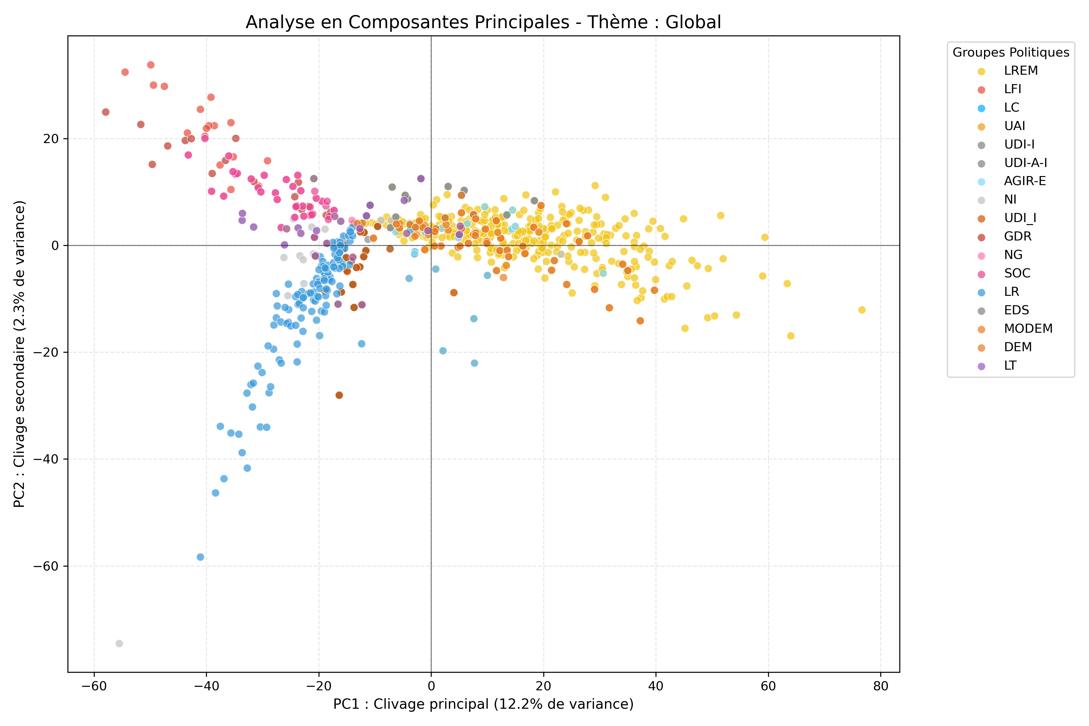 | 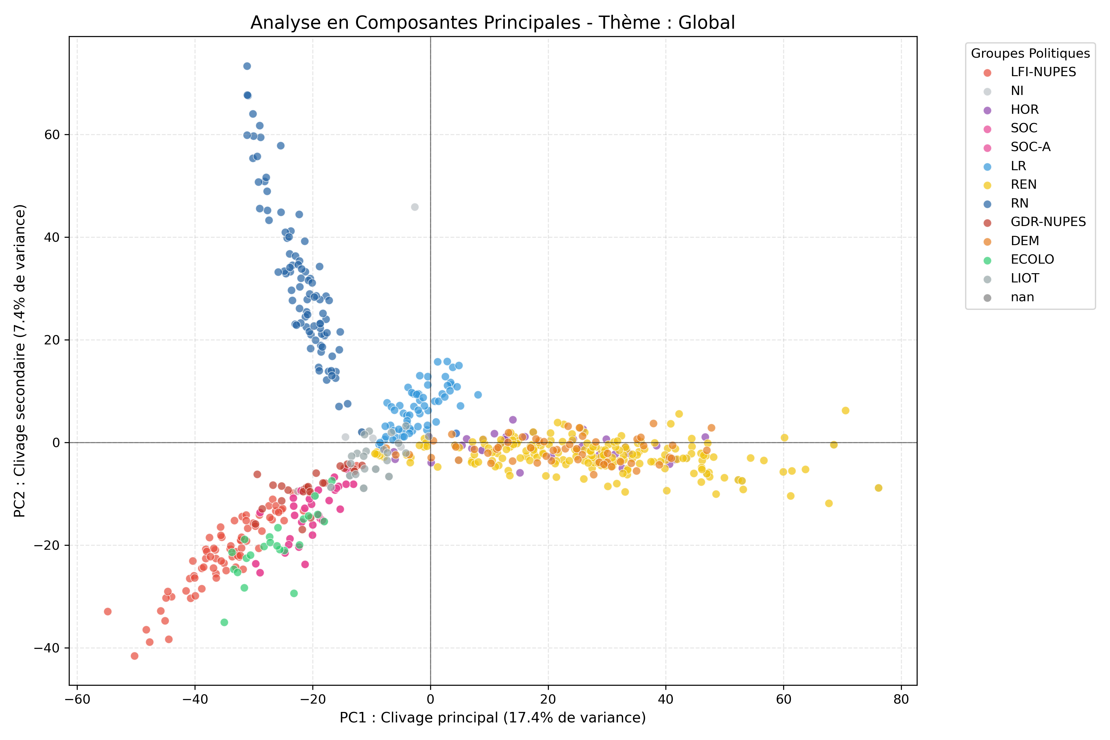 |
Figure 3: Principal Component Analysis for all ballots.
4.3 Thematic analysis
We apply a thematic classification based on the title of each ballot vote. Themes include:
- Ecology & Territories (agriculture, climate, energy, transport)
- Economy & State (taxation, customs, inflation)
- Security & International Affairs (police, justice, defense)
- Solidarity & Social Policy (pensions, social benefits, disability)
This enables theme-based analyses.
Categorization Methodology
We implemented a deterministic keyword-matching algorithm. This process filters the legislative titles provided by the NosDéputés.fr XML API to categorize each vote into one of four themes.
Methodological Note: While a Large Language Model (LLM) would undoubtedly be more “sophisticated” at interpreting the nuanced context of legislative titles, we decided to stick to a keyword-based approach. It is simple and easily understandable.
The script scans each titre (title) tag within the XML response. The ballot is mapped to the first theme, in the order below, with a keyword appearing in the title:
| |
Distribution of Ballots by Theme
The following table summarizes the volume of ballot votes analyzed for each legislature, categorized by the first matching theme. These themes serve as the basis for our comparative spatial analysis.
| Theme | 14th Legislature (2012-2017) | 15th Legislature (2017-2022) | 16th Legislature (2022-2024) |
|---|---|---|---|
| Solidarity & Social | 138 | 757 | 335 |
| Ecology & Territories | 73 | 641 | 709 |
| Economy & State | 72 | 157 | 68 |
| Security & International | 26 | 396 | 519 |
| Total Analyzed Ballots | 309 | 1,951 | 1,631 |
Our data contains 1,023 ballots for the 14th Legislature (2012–2017), 4,394 for the 15th (2017–2022) and 4,029 for the 16th (2022–2024, two years).
PCA by Theme
Beyond the global PCA, we repeat the analysis for each thematic domain. For example, for “Solidarity & Social”:
- Filter $\mathbf{M}$ to retain only ballot votes labeled “solidarity” or “social”
- Reapply PCA to this submatrix
- Visualize: Points colored by political group
- Compare the positions of the groups
The share of variance explained by PC1 differs between themes. It should be compared with care: it also depends on the number of ballots and differs between legislatures for all ballots taken together.
| 15th Legislature (2017-2022) | 16th Legislature (2022-2024) |
|---|---|
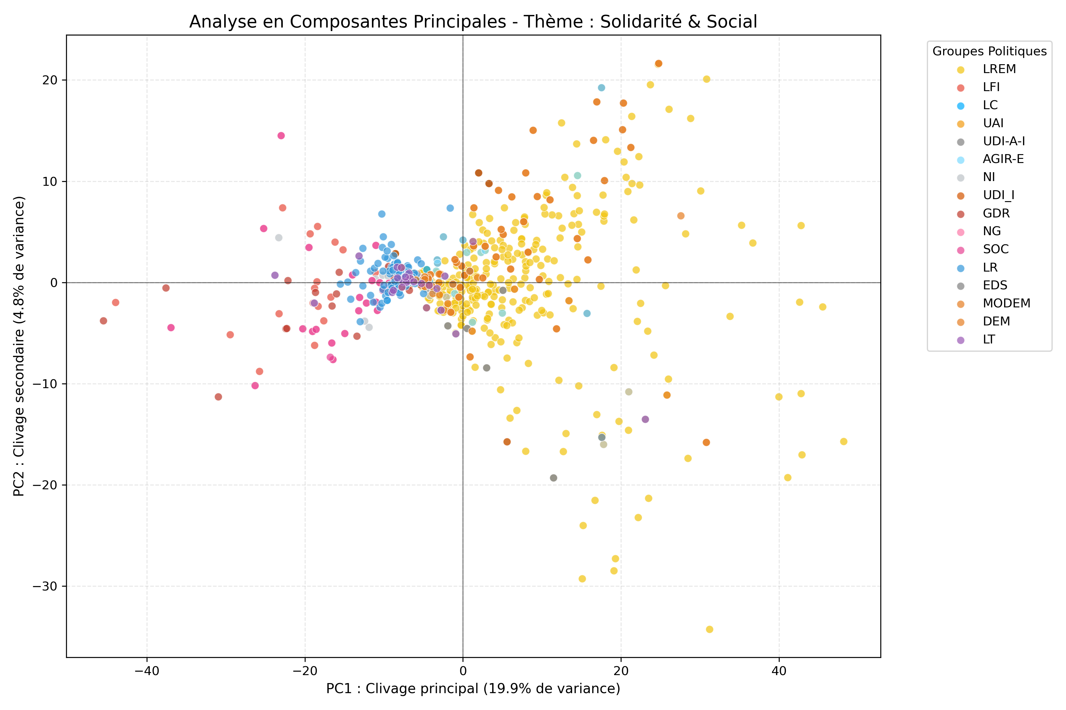 | 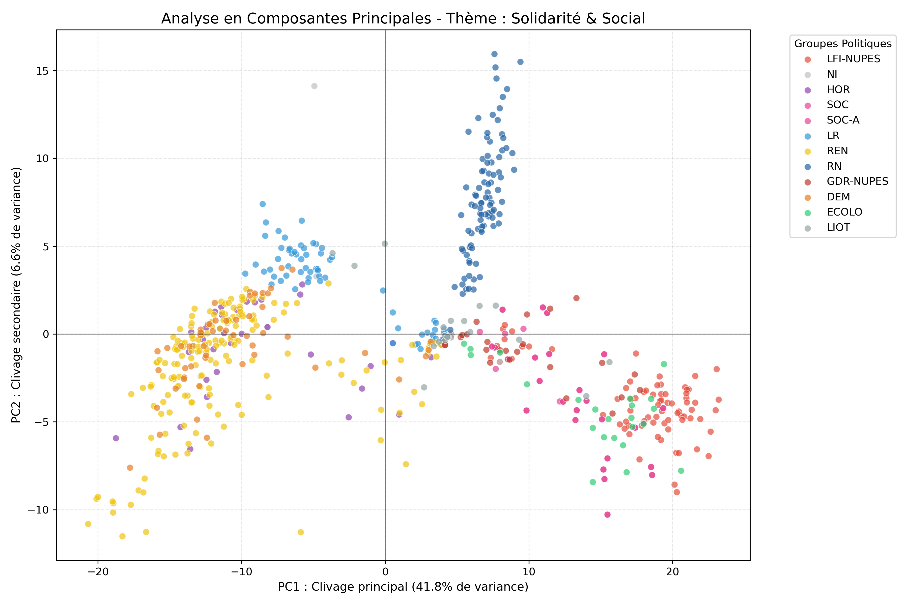 |
Figure 4: Principal Component Analysis for ballot votes related to Solidarity and Social.
Main observations:
15th Legislature (757 ballots). PC1 explains 19.9% of the variance. LFI, SOC and GDR are at one end, LREM at the other, and LR lies in between, close to the centre.
16th Legislature (335 ballots). PC1 explains 41.8% of the variance, against 17.4% for all the ballots of the same legislature (Figure 3). On these votes a single axis captures more than twice the share it captures overall, and the groups fall into three clearly separated areas: REN, DEM, HOR and LR at one end; LFI-NUPES, SOC-A and the ecologists at the other, with GDR between them; and the RN on the same side of PC1 as the left groups, but held apart from them by PC2.
5. Pivots: betweenness centrality
In addition to PCA, we compute the Betweenness Centrality of each MP in the k-NN graph.
Unlike degree, which counts an MP’s links, this metric counts how often an MP lies on the shortest paths between other MPs.
5.1. Definition
The centrality $g(v)$ of an MP $v$ is calculated by counting how many shortest paths between all other pairs of MPs pass through $v$:
$$g(v) = \sum_{s \neq v \neq t} \frac{\sigma_{st}(v)}{\sigma_{st}}$$Where:
- $\sigma_{st}$ is the total number of shortest paths from MP $s$ to MP $t$.
- $\sigma_{st}(v)$ is the number of those paths that pass through $v$.
5.2. Distance inversion and pathfinding
Since our graph edges represent similarity (Cosine Similarity), we must transform them into distances to find shortest paths. We define the distance $d_{ij}$ as:
$$d_{ij} = \frac{1}{\text{weight}_{ij} + \epsilon}$$This inversion ensures that a high voting similarity results in a short distance. We call “pivots” the MPs with the highest betweenness: they lie on many of the shortest paths between other MPs, including between clusters.
5.3. Results
Betweenness describes the position of an MP in the similarity graph. It is not a measure of political influence.
| Rank | 15th Leg. (2017-2022) | Group | 16th Leg. (2022-2024) | Group | |
|---|---|---|---|---|---|
| 1 | Jean-Luc Warsmann | UDI_I | Nathalie Bassire | LIOT | |
| 2 | Karine Lebon | GDR | Emmanuelle Ménard | NI | |
| 3 | Jennifer De Temmerman | LT | Jean-Carles Grelier | REN | |
| 4 | Thierry Michels | LREM | Olivier Serva | LIOT | |
| 5 | Agnès Thill | UDI_I | Jean-Victor Castor | GDR | |
| 6 | Lise Magnier | AGIR-E | Mansour Kamardine | LR | |
| 7 | Jean-Philippe Nilor | GDR | David Habib | NI | |
| 8 | Charles de Courson | LT | Charles de Courson | LIOT | |
| 9 | Brigitte Bourguignon | LREM | Victor Catteau | RN | |
| 10 | Paul Christophe | AGIR-E | Laurent Panifous | LIOT |
In the 16th Legislature, four of the ten pivots are LIOT MPs and two are non-attached (NI). In the 15th, the ten pivots come from five groups, two from each (UDI_I, GDR, LT, LREM, AGIR-E).
6. Conclusion
Main observations
- PC1 separates the groups of the presidential majority from the opposition groups, in both the 15th and the 16th Legislatures. It explains 12.2% and 17.4% of the variance.
- PC2 separates LFI and GDR from LR in the 15th Legislature, and the RN from LFI and the ecologists in the 16th.
- Participation shapes the plots: MPs who vote on few ballots are close to the point where an MP with no recorded vote would land.
Limitations
PC1 and PC2 together explain 14.5% of the variance in the 15th Legislature and 24.8% in the 16th. The other components are not analyzed here.
Reproducibility
The full source code is available in the GitHub repository: Networks-Analysis
References & Data Sources
NosDéputés.fr API https://www.nosdeputes.fr/api/
Provides access to parliamentary activities and metadata.Assemblée Nationale Open Data Portal https://data.assemblee-nationale.fr/
Official repository for voting records, law proposals, and legislative history.
Appendices
Appendix A: Intra-Group Analysis
For each political group $P$, we compute two distinct metrics:
Cohesion Leader (Intra-Group):
- Restrict the graph to members of $P$ only
- Identify the node with the maximum weighted degree in this subgraph
- This is the MP with the largest sum of similarity weights to the members of their own group they are linked to.
Hub Leader (Global):
- Identify the node from the group with the maximum weighted degree in the full graph
- The weighted degree adds up the similarity weights of all the MP’s links: to their own 5 nearest neighbours, and to the MPs who have them among theirs.
| Group | Cohesion Leader (Intra) | Hub Leader (Global) |
|---|---|---|
| LREM | Marie-Christine Verdier-Jouclas | Marie-Christine Verdier-Jouclas |
| LR | Bernard Deflesselles | Bernard Deflesselles |
| SOC | Christine Pires Beaune | Christine Pires Beaune |
| LFI | Mathilde Panot | Mathilde Panot |
Figure 5: Key Leaders for the 15th Legislature
| Group | Cohesion Leader (Intra) | Hub Leader (Global) |
|---|---|---|
| REN | Claire Guichard | Claire Guichard |
| RN | Victor Catteau | Victor Catteau |
| LFI-NUPES | Anne Stambach-Terrenoir | Anne Stambach-Terrenoir |
| LR | Jean-Jacques Gaultier | Michel Herbillon |
Figure 6: Key Leaders for the 16th Legislature
Participation of the leaders
- Claire Guichard (REN) and Victor Catteau (RN) voted on 66% and 57% of the ballots of the 16th Legislature, and Marie-Christine Verdier-Jouclas (LREM) on 44% of those of the 15th: among the highest values of their groups.
- The LR leaders voted on few ballots: Bernard Deflesselles on 4% in the 15th Legislature (LR median: 12%), Jean-Jacques Gaultier on 7% and Michel Herbillon on 5% in the 16th (LR median: 13%). The ballots they voted on have a high turnout (for Bernard Deflesselles, a median of 517 recorded voters, against 80 over all ballots), and they voted with the majority of their group 87% (Deflesselles) and 94% (Gaultier, Herbillon) of the time.
- Being a leader in the sense of weighted degree therefore does not require voting often.
Weighted degree describes the position of an MP in the similarity graph: it is not a measure of political influence.
Appendix B: Architecture and implementation of data retrieval
1 Data Source and API
Primary source: NosDéputés.fr, a freely accessible collaborative database, fed by the official data of the French National Assembly via its XML export protocols.
API endpoints:
| |
where LEGISLATURE $\in {15, 16}$ and SCRUTIN_ID is the numerical identifier of the vote.
Unfortunately, the API does not have as much data for previous legislatures. For the 14th legislature, we found an archive on Assemblée Nationale.
2 Parallel download protocol
To accelerate data collection (approx 4,000 ballot votes), we use a ThreadPoolExecutor with up to 10 concurrent workers.
Output: Three CSV files generated
dataset_scrutins_14.csv(2012–2017)dataset_scrutins_15.csv(2017–2022)dataset_scrutins_16.csv(2022–2024)
Each record: {depute, group, position, scrutin_id}
3 Transformation into a pivot matrix
The raw list of votes is transformed into a sparse matrix:
| |